Downloading and viewing deep dive

So far, we have gone through loading PDBs locally. This script walks you through the process of accessing a PDB from the internet without having to create a file.

Downloading and analyzing

import backmap
import requests # For accessing the PDB website
import io       # For treating a block text of text as a filehandle

# Identifying a PDB to view by its PDB ID
PDBID = "3E07"
PDBID = "8SHM"
PDBID = "1SP7"
PDBID = "2FFT"
# This is the structure of a URL that downloads a non-zipped PDB from RCSB.ORG
URL = f'https://files.rcsb.org/download/{PDBID}.pdb'
# "Downloading" (really, requesting)
response = requests.get(URL)#, stream=True)
# Accessing the PDB text
pdb_block = response.text

# Here, we could create a temporary file, save the text to the file
# and then provide the temporary filename to backmap, as done in the walkthrough
#with open('deme.pdb','wt') as f:
#   f.write(pdb_block)

# Instead of unnecessarily saving the file to your file system, you can use
# StringIO to convert the file into a filehandle
fh = io.StringIO(pdb_block)
# You can skip the next line, but then the PDB ID information will be missing
# in the graphs
fh.name = URL

# Analyzing the PDB and creating a new row "R"
structure_df = backmap.process_PDB(fh)
# Displaying the dataframe
structure_df.head()

	atomno	resname	chain	resid	occupancy	tf	segname	model	phi	psi	R
0	1	SER	A	1	1.0	2.00	None	1	NaN	29.085181	NaN
1	12	ALA	A	2	1.0	14.23	None	1	-161.710494	157.217687	0.493760
2	22	ALA	A	3	1.0	32.33	None	1	-163.929703	124.036378	0.444593
3	32	LYS	A	4	1.0	11.44	None	1	56.513637	-176.083053	0.333931
4	54	GLY	A	5	1.0	1.34	None	1	155.540044	-157.825870	0.496825

VIEWING SPECIFIC GRAPHS

So far, we have been using the backmap.draw_figures() function to view a set of figures (heatmaps showing per-residue R values, RMSD, RMSF, and per modle R histograms). In most situations, only some images may be, needed. In that situation, one could one of the four functions:

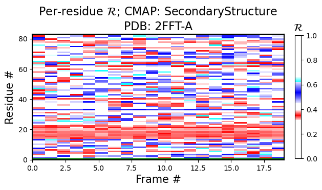
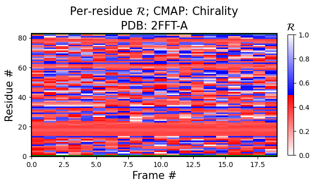
Per-model, per-residue R heatmaps

The following figure is colored by the SecondaryStructure cmap. But You can use Chirality, Greys, or any other legitimate cmap name available to matplotlib.

current_figures = backmap.draw_per_residue_plot(structure_df, output_dir='',
                                                write=False, show=True,
                                                v_limit = (0,1), cmap='SecondaryStructure')

# FOR REFERENCE: this is how we used to call all plots at once:
# should_be_true, figure_dict    = backmap.draw_figures(structure_df=structure_df, output_dir='',
#                                                       write=False, show=True)

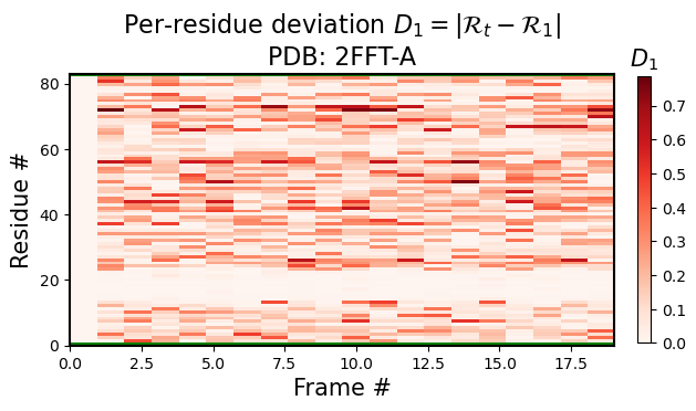
Per-model, per-residue RMSD(R) heatmaps

Here, for each model index \(t\), the per-residue \(RMSD(R)\) represents the root mean squared deviation of that model and residue’s R vs the first model and corresponding residue’s R (i.e., for any residue in model \(t\), the heatmap value would be represented by \(|R_t-R_1|\), where \(1\) represents the first model).

current_figures = backmap.draw_per_residue_RMSD(structure_df, output_dir='',
                                            write=False, show=True,
                                            v_limit = (0,1), cmap='Reds')

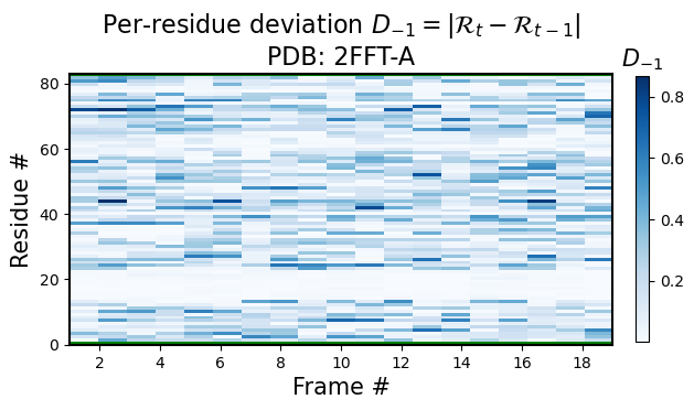
Identical to the function above, you can use the backmap.draw_per_residue_RMSF() function to get root mean squared fluctions; i.e., in stead of comparing corresponding residues between the current model \(t\) and the first model \(1\), one would compare to the previous model for any residue in model \(t\), the heatmap value would be represented by \(|R_t-R_{t-1}|\), where \(t-1\) represents the previous model.

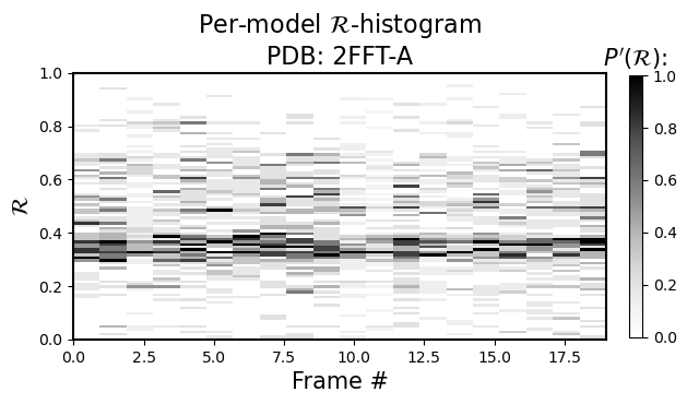
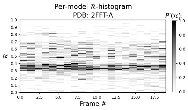
Per-model histograms of R

As the sub-title says, it allows you to see the histogram distribution of \(R\) for each model (so, \(R\) is now on the y-axis, and the color represents occupancy of the model’s residues in that regions of \(R\))

current_figures = backmap.draw_per_model_histogram(structure_df, output_dir='',
                                           write=False, show=True,
                                           bin_steps=0.2, v_limit = (0,1),
                                           cmap='Greys')

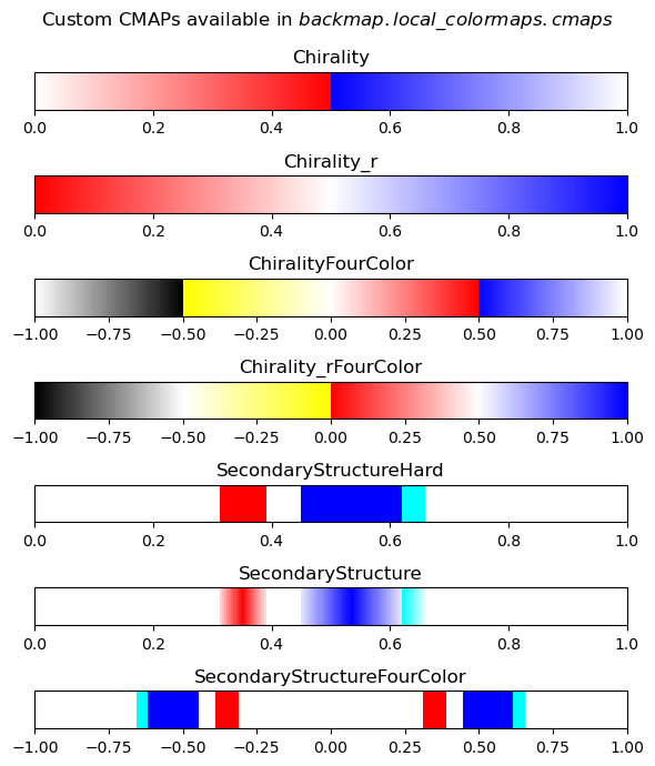
Displaying Custom Colormaps

Here are the custom color maps that are useful for displaying your own R-derived images. Their names should be identical to the names used for colormaps above

# Showing the types of colormaps available to backmap.local_colormaps

import backmap

fig,axes = backmap.local_colormaps.display_cmaps()

For completeness, using backmap.draw_figures()

This usage is identical to the one used in the first walkthrough notebook.

should_be_true, figure_dict    = backmap.draw_figures(structure_df=structure_df, output_dir='',
                                                       write=False, show=True)

<Figure size 640x480 with 0 Axes>