BackMAP EXAMPLES

Calculating Ramachandran numbers from phi, psi angles

Firstly, the Ramachandran number is easy to calculate if you already have each residue’s \(Φ\) (phi) and \(Ψ\) (psi) values.

E.g.:

import backmap
phi=110
psi=100
R_local = (phi+psi+360)/720.0

# Showing that this is the same as backmap.R()
assert backmap.R(phi=phi,psi=psi) == R_local

The equation above (\((\phi+\psi+360)/720\)) was derived in Mannige, 2018. The next notebook that shows how the proof was derived.

Using BackMAP to extract per-residue descriptors without displaying them

\(Φ\) (phi) and \(Ψ\) (psi) values are hard to calculate on the fly. If per residue phi, psi, and Ramachandran (R) numbers alal you need, then use backmap.process_PDB().

Here is an example (1MBA) of a simple PDB that has only one structure:

# A single PDB file with only one structure in it; note the model column that only contains the number 1
pdbfn = '../tests/pdbs/1mba.pdb'
structure_df1 = backmap.process_PDB(pdbfn)
print(f"{pdbfn} starts with:")
display(structure_df1.head(2))
print(f"...and ends with:")
structure_df1.tail(2)

../tests/pdbs/1mba.pdb starts with:

	atomno	resname	chain	resid	occupancy	tf	segname	model	phi	psi	R
0	4	SER	A	1	1.0	33.28	None	1	NaN	177.269699	NaN
1	10	LEU	A	2	1.0	20.17	None	1	-100.452393	162.714546	0.586475

...and ends with:

	atomno	resname	chain	resid	occupancy	tf	segname	model	phi	psi	R
144	1077	GLY	A	145	1.0	17.51	None	1	109.263031	1.896584	0.654388
145	1081	ALA	A	146	1.0	26.43	None	1	-142.910634	NaN	NaN

And here is an example (2fft) of a single PDB containing 20 structures (separated by the MODEL keyword):

# A more complicated PDB, with multiple models
import backmap
pdbfn = '../tests/pdbs/2fft.pdb.gz'
structure_df2 = backmap.process_PDB(pdbfn)
print(f"{pdbfn} starts with:")
display(structure_df2.head(2))
print(f"...and ends with:")
structure_df2.tail(2)

../tests/pdbs/2fft.pdb.gz starts with:

	atomno	resname	chain	resid	occupancy	tf	segname	model	phi	psi	R
0	1	SER	A	1	1.0	2.00	None	1	NaN	29.085181	NaN
1	12	ALA	A	2	1.0	14.23	None	1	-161.710494	157.217687	0.49376

...and ends with:

	atomno	resname	chain	resid	occupancy	tf	segname	model	phi	psi	R
1678	1209	LYS	A	83	1.0	44.30	None	20	-73.415831	159.043977	0.618928
1679	1231	ASP	A	84	1.0	21.33	None	20	-66.013609	NaN	NaN

Bonus: marking specific residues

# You can create a new boolean column called "mark" to mark any residues
# that you might want to. These residues will have a black square next to
# them adjacent to the right y axis

# Marking all lycines (normally, you would want to mark something more specific)
structure_df1['mark'] = False
structure_df1.loc[structure_df1['resname']=='LYS','mark'] = True

structure_df2['mark'] = False
structure_df2.loc[structure_df2['resname']=='LYS','mark'] = True

# Check in the display section to see the relevant residues marked
# (in the per-residue graphs) to the right of the main graph
# and to the left of the color bar.

Displaying structures and ensembles

Sometimes, displaying these structures can reveal interesting features quickly

For a detailed discussion on these graphs, refer to the downloading and viewing python notebook

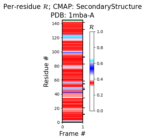
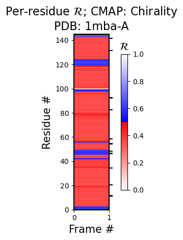
A slightly boring example: 1MBA

For example, for PDB ID 1mba, the second figure under heading 1 immediately reveals that the protein is dominantly alpha helical.

success, figure_dict = backmap.draw_figures(structure_df=structure_df1,
                                            output_dir=None,
                                            write=False,
                                            show=True)

        Chain "A" has only one model. Not drawing this graph.
        Chain "A" has only one model. Not drawing this graph.

<Figure size 640x480 with 0 Axes>

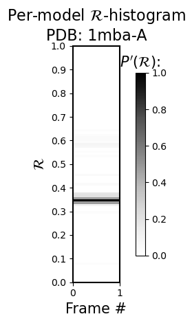
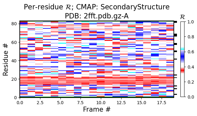
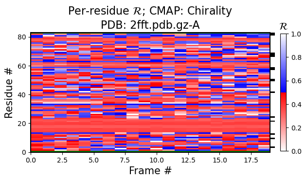
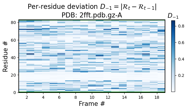
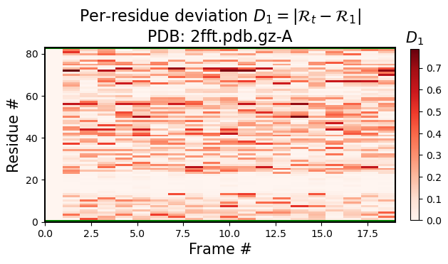
A more interesting structure: 2FFT

Note that looking at just one structure does not matter much, however, if you look at ensembles, then the value of the Ramachandran number is more visible.

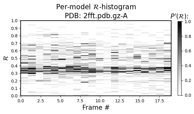
For example, the black-and-white histogram (Fig 1) shows that there is a single stable segment of the protein around residue number 20, which turns out to be an alpha helix.

Also, the same figure shows an interesting stable point at residue numbe 60. If there were two stable sections in a protein, you would only visualize the first or the second section by aligning all structures to that sections, but, given that their relative positions are always fluctuating due to the variable regions, you can not align both section together (also see 3 and 4).

success, figure_dict = backmap.draw_figures(structure_df=structure_df2,
                                            output_dir=None,
                                            write=False,
                                            show=True)

<Figure size 640x480 with 0 Axes>

Credit: I used the following tutorial to integrate python notebooks (originally available in backmap/notebooks/) into Sphinx documentation:

https://cybergis.github.io/github-pages-demo/tutorial/nbsphinx.html